Understanding Data in Data Science – Statistical Inference

In my previous posts in this series, I wrote on the analysis of single variables and multiple variables. The measures described in the previous posts apply to the entire known population, as well as random samples of the population. However, an additional challenge is introduced with random sampling – how do we tell if the sample mean, median, or correlation is representative of the entire population? This is a common problem in the world of data science.

Let’s try and understand this with an example: suppose you have 10 pumpkins that weigh 10, 9, 15, 11, 10, 9, 10, 12, 14, 500 pounds each. If you did a random sampling of 3 pumpkins and you picked the ones that weighed 12, 14, and 500 pounds, what would you say is more representative – the average (175 pounds) or median (13 pounds)?

In this case, you are able to see the entire population, so it is obvious that the median is more representative. On the other hand, if there were a thousand pumpkins and you did a random sampling of 10 pumpkins, how would you tell if the average or median is a better representation? This is what Statistical Inference tries to answer – what is a good statistic for the sample that describes the population and how accurate is that statistic?

Measures

The statistic used for the estimation (like mean or median) is called an estimator. There are different measures based on the chosen estimator.

Mean Squared Error (MSE)

If the estimator is the sample mean, it will minimize the MSE if there are no outliers. The MSE is computed as:

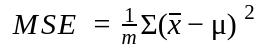
where m is the number times the random sample is drawn (attempts).

The Root Mean Square Error (RMSE) is the square root of the MSE. If there are outliers in the distribution, the MSE will not minimize after a certain number of attempts.

Estimated Variance

If the estimator is variance, the standard variance formula turns out to be a biased estimator for small samples. A simple change of the denominator from n to n – 1 makes it unbiased.

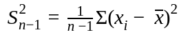
An unbiased estimator incrementally reduces the mean error to 0 with an increasing number of attempts.

Sampling Distribution

Continuing with our pumpkin example, let us say you decide to go with a sample mean weight of 11 pounds and sample standard deviation of 2 pounds (after factoring the 500 pound pumpkin as an outlier). If you are unlucky and picked the lightest pumpkins, this estimate could be way off. The variation in the estimate caused by random selection is called a sampling error. A sampling error is inevitable in inferring properties of a population and it may not be feasible to minimize it beyond a certain point. This makes it important to answer the question – if the sampling is repeated many times over, how would the estimates vary?

A sampling distribution can constructed with the estimated parameters. The following code snippet computes a sampling distribution from the sample mean and standard deviation of our pumpkin example:

import numpy as np
import math
import matplotlib.pyplot as plt

def sampling_distibution(mu, sigma, n=9, m=1000):
    """
    Generates a sampling distribution and
    computes the Standard Error (se) and Confidence Interval (ci)
    """
    means = [np.mean(np.random.normal(mu, sigma, n)) for _ in range(m)]
    ci = np.percentile(means, [5, 95]) # Confidence Interval: 5th & 95th percentile
    stderr = math.sqrt(np.mean([(x - mu)**2 for x in means])) # RMSE
    return (stderr, ci, means)

def plot_sampling_distribution(xs, nbins=500):
    """
    Generates a plot of the sampling distribution.
    
    A Cumulative Distribution Function (CDF) evaluated at x, is the probability
    of having values in the sample less than or equal to x.
    """
    (_, _, _) = plt.hist(xs, nbins, normed=1, histtype='step', cumulative=True)
    plt.title('Sampling distribution')
    plt.xlabel('Sample mean') 
    plt.ylabel('CDF')
    plt.show()

The sampling distribution is represented by the following plot:

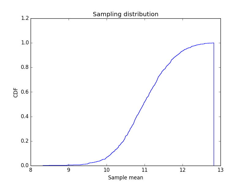
The sampling distribution computes two summaries – Standard Error and Confidence Interval.

Standard Error

This is the standard deviation of the sampling distribution of a statistic or a measure of how much we would expect the estimated mean to vary if we repeated the sampling process many times over. For our pumpkin example, the standard error (SE) comes to around half a pound, which means you can expect an estimate to be off by half a pound.

Confidence Interval

The confidence interval is a range that includes a given fraction of the sampling distribution. For example, a 90% confidence interval is the range from the 5th percentile to the 95th percentile. The smaller the confidence interval, the smaller the estimated variation with multiple re-sampling. For the pumpkin example, the confidence interval is roughly (10, 12). This means that the minimum weight is estimated to be 10 pounds and the maximum is estimated at 12 pounds.

Conclusion

This wraps up the first part of statistical inference methods. In the next part, I will explain Hypothesis Testing.