Introduction

Retail stores constantly gather purchase history and demographic data from their customers. Machine learning algorithms could use this data to give decision makers key insights about their customers. These algorithms are divided into three categories: supervised, unsupervised, and reinforcement learning. For this case study, we’ll be focusing on the first two. Supervised learning allows us to make a prediction based upon existing data, whereas unsupervised learning clusters the data population into different groups.

Understanding a business’ customers begins by segmenting the customer population into different groups based on shared characteristics. How these groups form will depend upon each business’ goals and their available data sets. Customer segmentation will let us form insights, such as customer lifetime value and purchase channel, so the business can use that information to drive future decisions.

About Data set

We sourced our data set from an online archive. The data set is transnational and contains a set of transactions from a UK registered and non-retail store. Many customers of the company are wholesalers. The data set in full can be accessed here: https://archive.ics.uci.edu/ml/datasets/Online+Retail

Attribute Information:

Customer value

Customers are segmented based on the business’ need and their available data. A few common customer segmentations include sorting by demographics or purchase history.

The data above only contains information about customer purchases. Based upon this set, we concluded that the most valuable method for customer segmentation would be customer value. This will allow us to identify the group of customers who have made the majority of this business’ purchases.

While there are several ways to identify customer value, here we’ll demonstrate RFM:

• Recency – How recently did the customer purchase?
• Frequency – How often do they purchase?
• Monetary Value – How much do they spend?

Data Preparation and Preprocessing

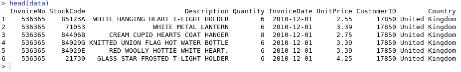
Below is the sample data from the original data set.

First, we used imputation techniques to remove special characters from numeric attributes. We also removed the largest values, the smallest values and outliers. Then, we processed the data to produce a data-frame that includes the frequency and monetary attributes. For now, we are excluding recency because its value, between 0-365, is not a continuous variable.

A set of R functions is created to implement the Independent FM scoring for each customer. For more information on this specific process, visit: https://github.com/3PillarGlobal/ds-cust-segmentation

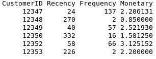
A new dataset is created with four columns: CustomerID, Recency, Frequency, and Monetary. The number in the Frequency column is the quantity of transactions a customer made during the period from StartDate to EndDate. The number in the Monetary column is the average amount of money per transaction during the same period.

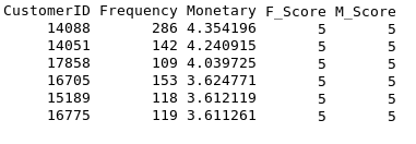
The data is further processed so that out of the scoring variables, the Recency, Frequency, and Monetary values represented by r, f, and m in aliquots independently, we calculate new attributes “F_Score”,”M_Score”.

Clustering and Visualization

The data for Frequency has high values, while Monetary, which is the Average monetary value, is somewhat smaller in comparison.

The data needs scaling in order for it to be properly represented graphically. This can be done through the following function in R code:

normalize <- function(x) {

 return ((x – min(x)) / (max(x) – min(x)))

}

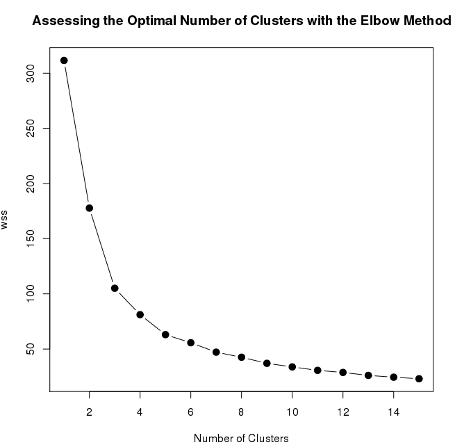
Below is the line graph that depicts the number of clusters needed for the k-means algorithm. It is the graph between WSS (standard error) and the number of clusters. After the number of clusters reaches 8, there is no change in values of standard error, even after the number of clusters increases. This means that we will have 8 clusters for our k-mean algorithm.

After applying the k-means clustering with the initial 8 clusters and 1000 number of iterations, we can segregate the customer based on the FM score. The following image is a visualization of how the data is segregated in different clusters.

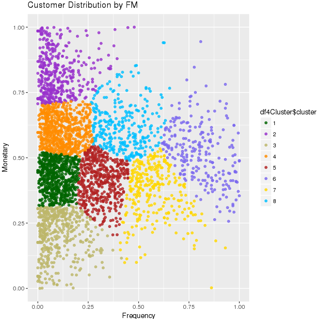
Conclusion

Data is scaled for both frequency and monetary value and eight different clusters are created by k-means algorithm shown by eight different colors in the graph above. Each portion (cluster) gives the idea for the value of the customer on the basis of their frequency and monetary in the retail data set.

This graph shows that the points highlighted with purple (having cluster number 6) at the top right are the most valuable customers because they display both high frequency and monetary value. Please note, however, that the above values are scaled down.

Clustering offers a fantastic opportunity for feature engineering.

Feel free to drop in your comments, suggestions, and share your experience while dealing with clustering problems.